PCA for Face Recognition
In this notebook, we will discuss a popular approach to face recognition called eigenfaces. The essence of eigenfaces is an unsupervised dimensionality reduction algorithm called Principal Components Analysis (PCA).
Dataset: We will take a subset of images from the famous Yale faces dataset. For analysis, we will use images for Subject 1 and Subject 14. For each subject, we will use 10 images to train the model and then 1 test image to perform face recognition and understand the results.
# Load Libraries
import numpy as np
import glob
from PIL import Image
import matplotlib.pyplot as plt
Explore Images for Subject 1 and 14
In this section, we will load and view original images of both subjects. We will reduce the size of these images to make our computation faster for the analysis and then view reduced images
Read Images for Subject 1
# Load Images for Subject 1
sub1images = glob.glob('yalefaces/subject01.*.gif')
print('Number of Images', len(sub1images))
# Plot original images
print('Original Images - Subject 1')
for i in range(len(sub1images)):
    im = Image.open(sub1images[i])
    plt.subplot(3,4,i+1)
    plt.imshow(im, cmap='gray')
    plt.xticks([])
    plt.yticks([])
plt.show()

# Check size of a random original image
orig_size = np.array(Image.open(sub1images[0]))
print(orig_size.shape)
Downsize Images
down_sub1images = []
for i in range(len(sub1images)):
    im = Image.open(sub1images[i])
    im = im.resize((im.size[0] // 4, im.size[1] // 4), Image.ANTIALIAS)
    down_sub1images.append(im)
    plt.subplot(3,4,i+1)
    plt.imshow(im, cmap='gray')
    plt.xticks([])
    plt.yticks([])
plt.show()

# Check size of downsized image
dwn_size = np.array(down_sub1images[0])
print(dwn_size.shape)
Read Images for Subject 14
# Load Images for Subject 1
sub14images = glob.glob('yalefaces/subject14.*.gif')
print('Number of Images', len(sub14images))
# Plot original images
print('Original Images - Subject 14')
for i in range(len(sub14images)):
    im = Image.open(sub14images[i])
    plt.subplot(3,4,i+1)
    plt.imshow(im, cmap='gray')
    plt.xticks([])
    plt.yticks([])
plt.show()

# Check size of a random original image
orig_size = np.array(Image.open(sub14images[0]))
print(orig_size.shape)
Downsize Images
down_sub14images = []
for i in range(len(sub14images)):
    im = Image.open(sub14images[i])
    im = im.resize((im.size[0] // 4, im.size[1] // 4), Image.ANTIALIAS)
    down_sub14images.append(im)
    plt.subplot(3,4,i+1)
    plt.imshow(im, cmap='gray')
    plt.xticks([])
    plt.yticks([])
plt.show()

# Check size of downsized image
dwn_size = np.array(down_sub14images[0])
print(dwn_size.shape)
Plot Mean Faces
Mean Face is the average face of all images. In this section we will plot the mean face of downsized images for both Subject 1 and Subject 14.
Flatten Images
To create an average face, we will first need to flatten the images.
# Flatten Images for Subject 1
flt_sub1img = np.asarray([np.array(img).flatten() for img in down_sub1images])
print('Shape of Sub1 Flat image matrix is: ', flt_sub1img.shape)

flt_sub14img = np.asarray([np.array(img).flatten() for img in down_sub14images])
print('Shape of Sub14 Flat image matrix is: ', flt_sub14img.shape)
Plot Mean Faces
# Mean Face of Subject 1
mean_face = np.zeros((1,60*80))
for i in flt_sub1img:
    mean_face = np.add(mean_face, i)

mean_face = np.divide(mean_face, float(len(down_sub1images))).flatten()
plt.imshow(mean_face.reshape(60,80), cmap='gray')
plt.show()

# Mean Face of Subject 14
mean_face = np.zeros((1,60*80))
for i in flt_sub14img:
    mean_face = np.add(mean_face, i)

mean_face = np.divide(mean_face, float(len(down_sub14images))).flatten()
plt.imshow(mean_face.reshape(60,80), cmap='gray')
plt.show()

Create Eigenfaces
In this section, we will plot eigenfaces. One of the simplest and most effective approaches used in face recognition systems is the so-called eigenface approach. This approach transforms faces into a small set of essential characteristics, eigenfaces, which are the main components of the initial set of learning images. To create eigenfaces, we will use PCA. PCA involves the following steps:
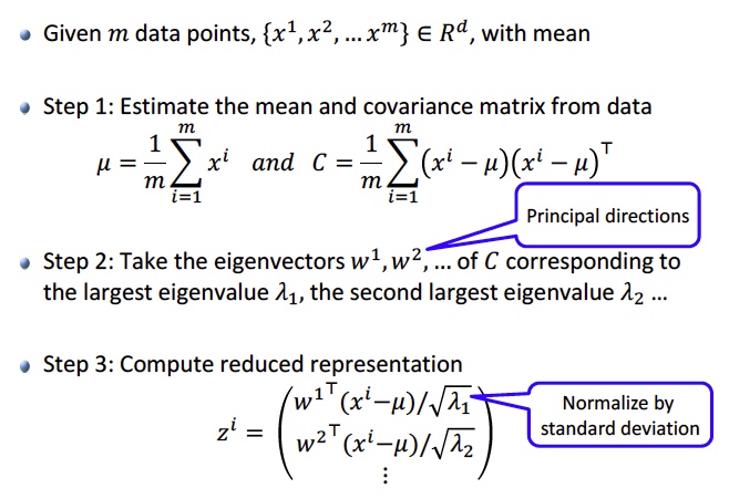 Image Source: Georgia Tech CSE 6740 Machine Learning course slides
Center Data
PCA requires that we center our data.
# Center Data
mean_sub1X = flt_sub1img.mean(axis=0)
sub1X = flt_sub1img - mean_sub1X
print('Shape of Sub1 centered data: ', sub1X.shape)

mean_sub14X = flt_sub14img.mean(axis=0)
sub14X = flt_sub14img - mean_sub14X
print('Shape of Sub14 centered data: ', sub14X.shape)
Create Covariance Matrix
# Create Cov matrix
sub1_cov_matrix = np.cov(sub1X)
print('Shape of Sub1 Covariance Matrix: ', sub1_cov_matrix.shape)

sub14_cov_matrix = np.cov(sub14X)
print('Shape of Sub14 Covariance Matrix: ', sub14_cov_matrix.shape)
Get Eigenvectors and Eigenvalues
 # Get Eigenvector and eigenvalues
sub1_eig_vals, sub1_eig_vecs = np.linalg.eigh(sub1_cov_matrix)
print('Sub1 First Eigenvector \n%s' %sub1_eig_vecs[0])
print('\nSub1 Eigenvalues \n%s' %sub1_eig_vals)
print('\n')
sub14_eig_vals, sub14_eig_vecs = np.linalg.eigh(sub14_cov_matrix)
print('Sub14 First Eigenvector \n%s' %sub14_eig_vecs[0])
print('\nSub14 Eigenvalues \n%s' %sub14_eig_vals)
Sort Eigenvectors and Check Variance Explained
Create pairs of Eigenvalues and Eigenvectors
# Subject 1
sub1_eig_pairs = [(sub1_eig_vals[index], sub1_eig_vecs[:,index]) for index in range(len(sub1_eig_vals))]

# Subject 14
sub14_eig_pairs = [(sub14_eig_vals[index], sub14_eig_vecs[:,index]) for index in range(len(sub14_eig_vals))]
Sort Pairs in Descending Order of Eigenvalues
# Subject 1
sub1_eig_pairs.sort(reverse=True)
sub1_eigvalues_sort  = [sub1_eig_pairs[index][0] for index in range(len(sub1_eig_vals))]
sub1_eigvectors_sort = [sub1_eig_pairs[index][1] for index in range(len(sub1_eig_vals))]

# Subject 14
sub14_eig_pairs.sort(reverse=True)
sub14_eigvalues_sort  = [sub14_eig_pairs[index][0] for index in range(len(sub14_eig_vals))]
sub14_eigvectors_sort = [sub14_eig_pairs[index][1] for index in range(len(sub14_eig_vals))]
Get Cumulative Variance Explained
# Subject 1
sub1_var = np.cumsum(sub1_eigvalues_sort)/sum(sub1_eigvalues_sort)

# Subject 14
sub14_var = np.cumsum(sub14_eigvalues_sort)/sum(sub14_eigvalues_sort)

# Show cumulative proportion of varaince with respect to components
print("Sub1 Cumulative proportion of variance explained vector: \n%s" %sub1_var)
print('\n')
print("Sub14 Cumulative proportion of variance explained vector: \n%s" %sub14_var)
Plot Eigenfaces
Choose Top 6 Eigenvectors
Here we choose the eigenvectors that explain most variation in our data. We will pick the top 6 eigenvectors.
#Choose necessary PC
sub1_reduced_data = np.array(sub1_eigvectors_sort[:6]).transpose()
print('Shape of Sub1 reduced data: ', sub1_reduced_data.shape)

sub14_reduced_data = np.array(sub14_eigvectors_sort[:6]).transpose()
print('Shape of Sub14 reduced data: ', sub14_reduced_data.shape)
Project on Eigenvectors
To create eigenfaces, we need to project our centered data onto the top 6 principal components we created.
# Project Data
sub1_proj_data = np.dot(sub1X.T,sub1_reduced_data)
sub1_proj_data = sub1_proj_data.transpose()
print('Shape of Sub1 Projected Data: ', sub1_proj_data.shape)

sub14_proj_data = np.dot(sub14X.T,sub14_reduced_data)
sub14_proj_data = sub14_proj_data.transpose()
print('Shape of Sub14 Projected Data: ', sub14_proj_data.shape)
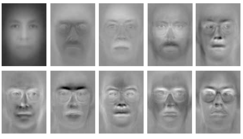
Plot Eigenfaces
# Subject 1
for i in range(sub1_proj_data.shape[0]):
    img = sub1_proj_data[i].reshape(im.size[1],im.size[0])
    plt.subplot(2,4,1+i)
    plt.imshow(img, cmap='gray')
    plt.xticks([])
    plt.yticks([])
#    plt.savefig('test1_eigenface.jpg')
plt.show()

Observations: The first eigenface, top-left, seems to be the most representative of the original images. The background has different levels of illumination, and the face is recognizable. Subject 1’s light skin and sharp facial features create a lot of illumination in the six eigenfaces.
The remaining eigenfaces seem are a combination of a few original images. The first image on the second row shows sleepy image above the nose and the happy image below. The last eigenface on the top row appears to be a combination between the surprised image above the nose, and the normal image below the nose. The last eigenface looks like a combination of the wink image above the nose, while the image is blurry below the nose. Glasses cannot be seen in any of the eigenfaces but could be because there is only 1 original image of subject 1 with glasses.
# Subject 14
for i in range(sub14_proj_data.shape[0]):
    img = sub14_proj_data[i].reshape(im.size[1],im.size[0])
    plt.subplot(2,4,1+i)
    plt.imshow(img, cmap='gray')
    plt.xticks([])
    plt.yticks([])
#    plt.savefig('test14_eigenface.jpg')
plt.show()

Observations: The first eigenface, top-left, seems to be the most representative of the original images. The background has different levels of illumination, and the face is recognizable. Glasses can be seen in the first eigenface which are present in some of subject 14’s images. Subject 14’s skin tone and facial features create little variations in the illumination of the images.
The remaining eigenfaces appear to be a combination of a few original subject images. The first image on the bottom row seems to be a combination of sleepy and happy image. The last eigenface looks like a combination of sleepy and sad images with no glasses. The last eigenface on the top row shows glasses. Surprised or wink expressions cannot be seen in any of these eigenfaces.
Face Recognition
To perform face recognition, we will project the test images on top eigenfaces. The idea is to generate a correlation score and identify if our algorithm would be able to recognize these images based ont he score generated.
To do this, we will:
- Load 2 test images (1 image for each subject)
- Downsize the images
- Center the images
- Project images on the top eigenface of each subject to generate a correlation score
Get and Plot Test Images
# Get Test images
testimg = glob.glob('yalefaces/subject??-test.gif')
len(testimg)
# Downsize and plot Test Images
test_images = []
for i in range(len(testimg)):
    im = Image.open(testimg[i])
    im = im.resize((im.size[0] // 4, im.size[1] // 4), Image.ANTIALIAS)
    plt.subplot(1,2,i+1)
    plt.imshow(im, cmap='gray')
    test_images.append(im)
plt.show()

# Check size of test images
test_size = np.array(test_images[1])
test_size.shape
Project Test Images
Here we will project the test images on top eigenfaces of each subject to obtain correlation score.
# Plot Eigenface of Subject 1
print('Top Eigenface of Subject 1')
eig1 = sub1_proj_data[0].reshape(im.size[1],im.size[0])
plt.imshow(eig1, cmap='gray')
plt.show()

# Project and create correlation score - Subject 1
print('Correlations scores with test images:')
for img in test_images:
    plt.imshow(img, cmap='gray')  # Plot test image
    plt.show()
    fltimg = np.asarray(np.array(img).flatten())  # Flatten test image
    norm_img = fltimg - mean_sub1X  # Center test image
    # Create Correlation score
    sub1_test = np.dot(sub1_proj_data[0].T, norm_img) / np.dot(np.linalg.norm(sub1_proj_data[0]), np.linalg.norm(norm_img))
    print('Correlation score for Eigenface of Subject 1 with Test Image shown \n', sub1_test)


Projecting test image of Subject 1 using eigenface of Subject 1: Based on the score (0.304), correlation between test image and eigenface seems to be low to moderately positively correlated. This low correlation could be because while test image has a white background, the eigenface has right side of its face illuminated, and left side is shadowed. The face recognition algorithm may be able to identify a face, but a low correlation score is not very promising and the algorithm may not identify subject 1’s face.
Projecting test image of Subject 14 using eigenface of Subject 1: Based on the score (-0.420), correlation between test image and eigenface seems to be low to moderately negatively correlated. There are differences in background illumination, hair, shape of the face and head and presence of glasses between the test image and eigenface. The face recognition algorithm may be able to identify a face, and a negative correlation could help discard non-matching faces.
# Plot Eigenface of Subject 14
print('Top Eigenface of Subject 14')
eig14 = sub14_proj_data[0].reshape(im.size[1],im.size[0])
plt.imshow(eig14, cmap='gray')
plt.show()

# Project and create correlation score - Subject 1
print('Correlations scores with test images:')
for img in test_images:
    plt.imshow(img, cmap='gray')  # Plot test image
    plt.show()
    fltimg = np.asarray(np.array(img).flatten())  # Flatten test image
    norm_img = fltimg - mean_sub1X  # Center test image
    # Create Correlation score
    sub14_test = np.dot(sub14_proj_data[0].T, norm_img) / np.dot(np.linalg.norm(sub14_proj_data[0]), np.linalg.norm(norm_img))
    print('Correlation score for Eigenface of Subject 14 with Test Image shown \n', sub14_test)

Projecting test image of Subject 1 using eigenface of Subject 14: Based on the score (-0.389), correlation between test image and eigenface seems to be low to moderately positively correlated. There are differences in background illumination, hair, shape of the face and head and presence of glasses between the test image and eigenface. The face recognition algorithm may be able to identify a face, but a low correlation score is not very promising and the algorithm may not identify subject 14’s face.
Projecting test image of Subject 14 using eigenface of Subject 14: Based on the score (0.558), correlation between test image and eigenface seems to be moderately correlated. This correlation could be because while test image has a white background, the eigenface has left side of its face illuminated, and right side is shadowed The face recognition algorithm may be able to identify a face, and a moderate correlation score may lead the algorithm to identify subject 14’s face.